Introduction to Topic Modelling in NLP

• Topic modelling is the study of patterns of word co-occurrence across documents to reveal underlying thematic structures that are not explicitly labeled or defined. This makes it especially useful for exploring large, unstructured corpora such as news articles, research papers, customer reviews, or social media data.
• Unlike classification models, topic modelling does not rely on pre-annotated/ labelled datasets. Instead, it learns directly from raw text, making it a practical choice when labeled data is insufficient, expensive to create, or unavailable.
• Topic modelling reflects real-world text more accurately by allowing each document to be represented as a mixture of topics rather than forcing it into a single category. For example, an article can discuss both “machine learning” and “healthcare,” with different proportions assigned to each topic.
• Each topic is defined by a set of related words, where each word is assigned a probability indicating its importance within that topic. This probabilistic representation helps interpret topics and understand which terms contribute most strongly to a given theme.
• LDA models documents as mixtures of topics and topics as mixtures of words using a well-defined probabilistic framework. Its interpretability, mathematical grounding, and wide library support have made it the standard baseline for topic modelling tasks across research and industry.

Modern applications generate massive amounts of unstructured text data, such as emails, reviews, articles, chat logs, and research papers. Manually organizing and understanding this data is impractical. Topic modelling helps structure this unorganized text by identifying themes that occur repeatedly across documents.

Another important reason topic modelling is useful is that traditional keyword search is often limited. Two documents may talk about the same idea using different words, and keyword-based methods may fail to connect them. Topic modelling goes beyond exact word matching and focuses on semantic patterns, making it more effective for understanding text at scale.

To understand topic modelling, it is important to understand how text is represented mathematically. Text data is first converted into numerical form, usually using a bag-of-words representation. In this representation, a document is treated as a collection of words where word order is ignored, but word frequency is preserved.

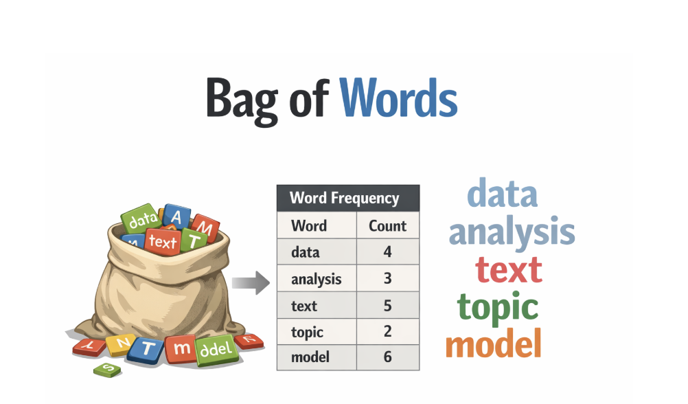
Each document is represented as a vector of word counts. Across a collection of documents, this forms a document-term matrix, where rows represent documents and columns represent words. Topic modelling algorithms analyze this matrix to find groups of words that frequently appear together.

A topic in topic modelling is not a single label but a probability distribution over words. Similarly, each document is represented as a probability distribution over topics. This means a document can talk about multiple topics with different proportions.

Latent Dirichlet Allocation, commonly known as LDA, is the most popular topic modelling algorithm. LDA is a probabilistic generative model that assumes documents are created through a hidden process involving topics.

LDA assumes that each document has a mixture of topics, and each topic has a mixture of words. When generating a document, the model first chooses a topic based on the document’s topic distribution and then chooses a word based on the topic’s word distribution. This process is repeated for every word in the document.

The “latent” part of LDA refers to the fact that topics are hidden and not directly observed. The model tries to infer these hidden topics from the observed words. The “Dirichlet” part refers to the Dirichlet distribution, which is used as a prior to control how topics are distributed across documents and how words are distributed across topics.

Setting up a tiny corpus

Assume a very small vocabulary of four words:

w₁ = “ai” w₂ = “data” w₃ = “pizza” w₄ = “pasta”

Now, assume we have three documents:

Document 1: “ai data ai” Document 2: “ai data data” Document 3: “pizza pasta pizza”

We convert this corpus into a document–term matrix X using raw word counts.

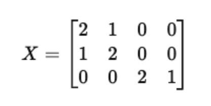
Each row is a document, each column is a word, and each entry is how many times that word appears in that document.

Choosing the number of topics

Assume K = 2 topics.

Topic 1 roughly corresponds to “technology” Topic 2 roughly corresponds to “food”

LDA does not know this in advance. We are assuming it here only to illustrate the learned matrices.

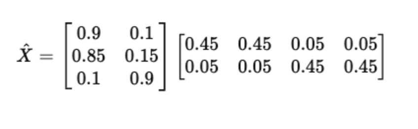
Topic–word matrix Φ (K × V)

Φ contains word probabilities for each topic. Each row sums to 1.

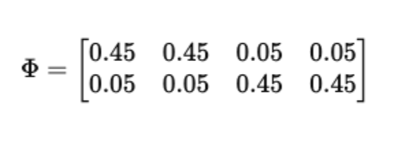
Interpretation:

For Topic 1 (technology): P(ai)=0.45, P(data)=0.45, P(pizza)=0.05, P(pasta)=0.05

For Topic 2 (food): P(ai)=0.05, P(data)=0.05, P(pizza)=0.45, P(pasta)=0.45

This matrix answers the question: given a topic, how likely is each word?

Document–topic matrix Θ (D × K)

Θ contains topic proportions for each document. Each row sums to 1.

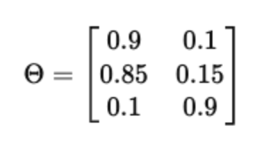
Interpretation:

Document 1 is 90% topic 1 and 10% topic 2 Document 2 is 85% topic 1 and 15% topic 2 Document 3 is 10% topic 1 and 90% topic 2

This matrix answers the question: given a document, how much does each topic contribute?

Matrix multiplication: reconstructing the corpus

LDA assumes the expected word distribution per document comes from:

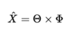
Let’s compute this explicitly.

Row-by-row multiplication

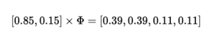
For Document 1:

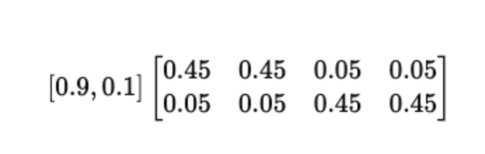
=[0.9(0.45)+0.1(0.05),0.9(0.45)+0.1(0.05),0.9(0.05)+0.1(0.45),0.9(0.05)+0.1(0.45)] =[0.41,0.41,0.09,0.09]= [0.41, 0.41, 0.09, 0.09]=[0.41,0.41,0.09,0.09]

This means document 1 is expected to heavily favor “ai” and “data”.

For Document 2:

Again, a strong technology signal with a small food component.

For Document 3:

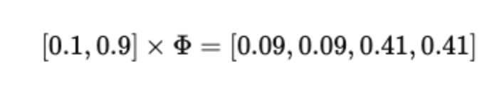
Clearly dominated by food-related words.

Final reconstructed matrix

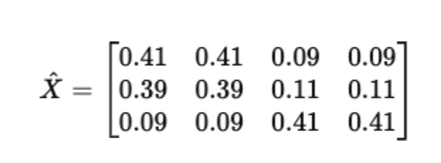
This matrix is a probabilistic approximation of the original count matrix X. LDA is effectively performing a constrained matrix factorization where all entries are non-negative, and rows of Θ and Φ are probability distributions.

During training, LDA does not directly compute Θ × Φ once. Instead, it repeatedly updates topic assignments for individual word occurrences so that the implied Θ and Φ make X likely under the generative model. Variational inference updates Θ and Φ directly using optimization.

Both methods aim to find Θ and Φ such that ΘΦ explains X well.

Python demo with matrices printed

Here is a Python example that explicitly prints Θ and Φ so you can inspect them.

import numpy as np

from sklearn.decomposition import LatentDirichletAllocation
from sklearn.feature_extraction.text import CountVectorizer

docs = [
    "ai data ai",
    "ai data data",
    "pizza pasta pizza"
]

vectorizer = CountVectorizer()
X = vectorizer.fit_transform(docs)

lda = LatentDirichletAllocation(
    n_components=2,
    random_state=0,
    max_iter=50
)

lda.fit(X)

# Document-topic matrix Θ
Theta = lda.transform(X)

# Topic-word matrix Φ (normalize rows)
Phi = lda.components_ / lda.components_.sum(axis=1)[:, None]

print("Vocabulary:", vectorizer.get_feature_names_out())
print("\nDocument-Term Matrix X:")
print(X.toarray())

print("\nDocument-Topic Matrix Θ:")
print(Theta)

print("\nTopic-Word Matrix Φ:")
print(Phi)

print("\nReconstructed X (Θ × Φ):")
print(np.dot(Theta, Phi))

You will see that Θ × Φ closely matches the structure of X, even though the values are probabilities rather than raw counts.

Probabilistic Latent Semantic Analysis (PLSA) extends the idea of latent semantic structure by introducing an explicit probabilistic latent variable model over documents and words. Given a document ddd and a word w, PLSA assumes their co-occurrence is generated through a latent topic variable z. The joint probability is defined as:

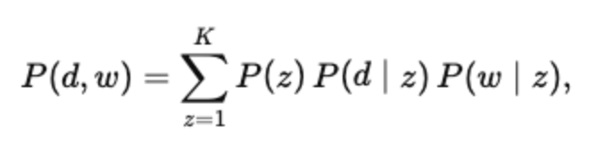
which can also be written in conditional form as:

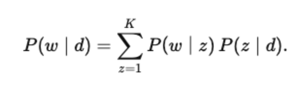
Here, P(w∣z) represents the topic–word distribution and P(z∣d) represents how strongly a topic contributes to a document. Model parameters are learned by maximizing the log-likelihood of the observed document–word counts n(d,w):

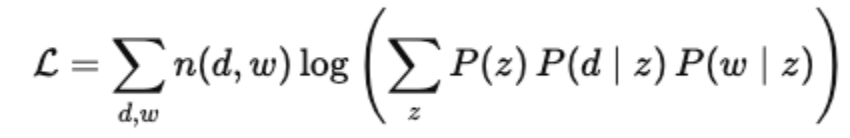
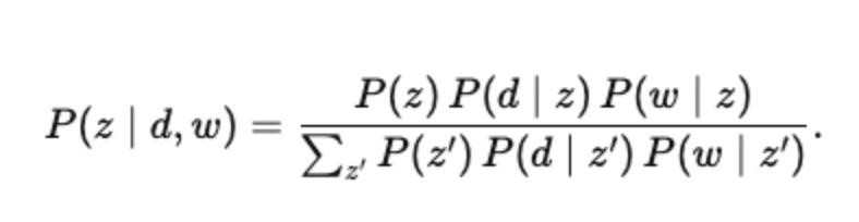
Because the topic variable z is unobserved, PLSA uses the Expectation–Maximization (EM) algorithm. In the E-step, posterior topic assignments are computed as:

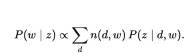
In the M-step, the topic–word and document–topic distributions are updated using these posteriors, for example:

PLSA can also be viewed as a probabilistic matrix factorization of the document–word distribution matrix P(d,w) into lower-rank factors corresponding to topics, similar in spirit to LSA but grounded in likelihood maximization rather than SVD.

Traditional topic models like LDA rely on word counts and probabilistic assumptions. BERT-based topic modeling works very differently.

Instead of modeling documents as bags of words, we first use a pretrained BERT model to convert each document into a dense semantic vector (embedding). Documents with similar meanings end up close together in vector space. Once we have these embeddings, we cluster them to find groups of semantically similar documents. Finally, we extract representative words for each cluster to describe the topic.

BERTopic combines four ideas:

BERT embeddings to capture semantics UMAP to reduce dimensionality HDBSCAN to cluster documents Class-based TF-IDF (c-TF-IDF) to extract topic words

Make sure you have these installed first.

pip install bertopic sentence-transformers scikit-learn datasets umap-learn hdbscan

We will use a subset of the 20 Newsgroups dataset, which is commonly used for topic modeling and text classification.

from bertopic import BERTopic
from sentence_transformers import SentenceTransformer
from sklearn.datasets import fetch_20newsgroups
from sklearn.feature_extraction.text import CountVectorizer
import pandas as pd

Step 1: Load a real dataset

docs = fetch_20newsgroups(
    subset="train",
    remove=("headers", "footers", "quotes")
).data
docs[0]

At this point, docs is a list of raw text documents. Each document may talk about technology, sports, religion, politics, or science.

I was wondering if anyone out there could enlighten me on this car I saw\nthe other day. It was a 2-door sports car, looked to be from the late 60s/\nearly 70s. It was called a Bricklin. The doors were really small. In addition,\nthe front bumper was separate from the rest of the body. This is \nall I know. If anyone can tellme a model name, engine specs, years\nof production, where this car is made, history, or whatever info you\nhave on this funky looking car, please e-mail.

Step 2: Load a BERT embedding model

embedding_model = SentenceTransformer("all-MiniLM-L6-v2")

This model converts each document into a 384-dimensional dense vector. These embeddings capture semantic meaning, not just word overlap.

Step 3: Initialize BERTopic

topic_model = BERTopic(
    embedding_model=embedding_model,
    vectorizer_model=CountVectorizer(stop_words="english"),
    language="english",
    calculate_probabilities=True,
    verbose=True
)

Here’s what is happening conceptually:

The BERT model generates document embeddings UMAP reduces embedding dimensions HDBSCAN clusters documents TF-IDF extracts representative topic words

Step 4: Fit the topic model

topics, probs = topic_model.fit_transform(docs)

This single line does a lot of work:

Each document is embedded using BERT Documents are clustered based on semantic similarity Each document is assigned a topic ID Topic probabilities are computed

topics contain one topic label per document.

Step 5: Inspect discovered topics

topic_info = topic_model.get_topic_info()
print(topic_info.head(10))

This shows:

Topic ID Number of documents in the topic Top representative words

Topic -1 represents outliers (documents that do not fit well into any topic).

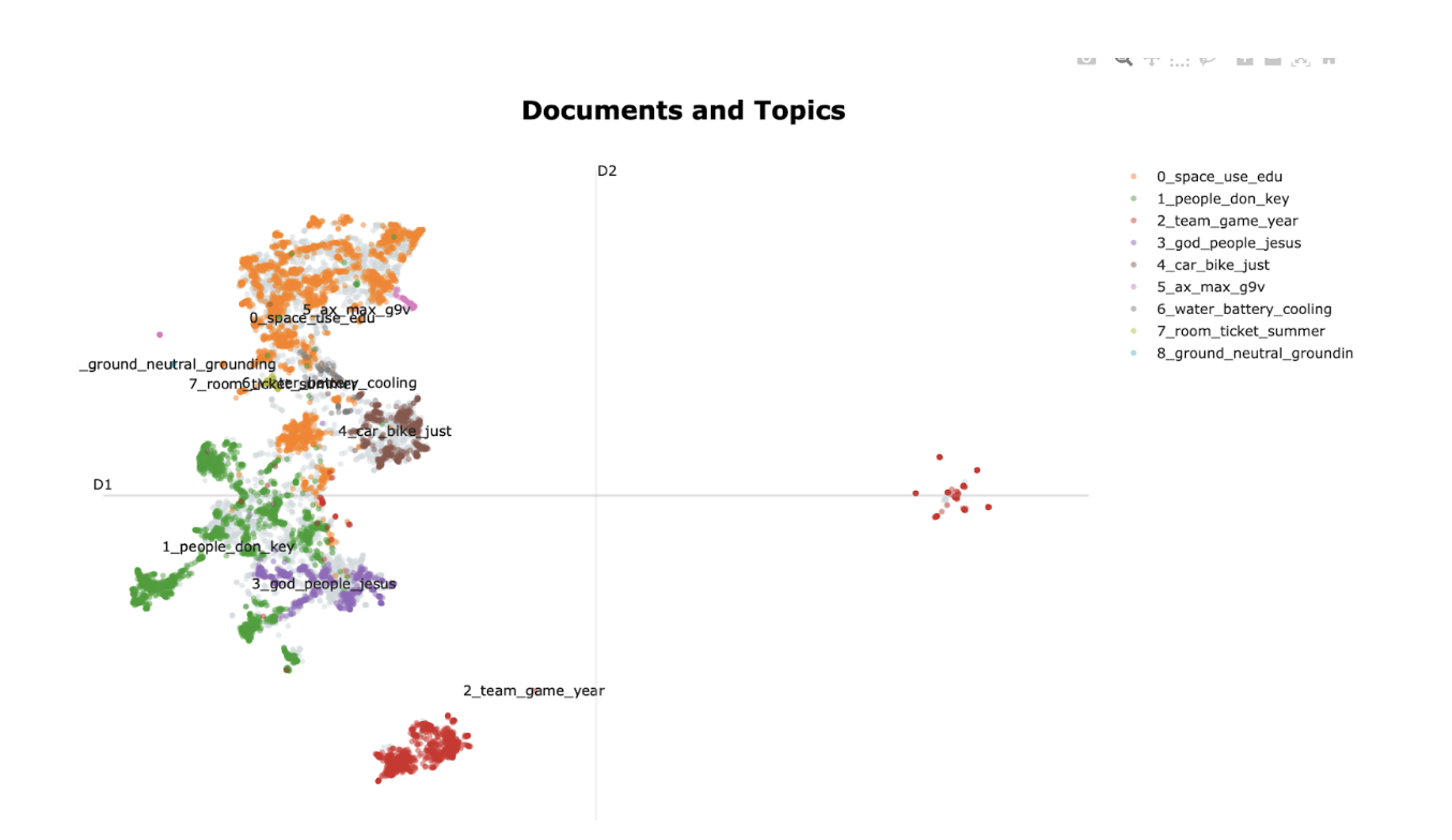
  Topic  Count                           Name  \
0     -1   3604             -1_god_db_like_don   
1      0   1074       0_team_game_season_games   
2      1    514  1_patients_msg_medical_health   
3      2    394      2_space_launch_nasa_orbit   
4      3    359  3_key_clipper_chip_encryption   
5      4    261       4_card_monitor_video_vga   
6      5    239     5_israel_israeli_arab_jews   
7      6    185             6_jpeg_image_cx_c_   
8      7    167     7_fbi_koresh_batf_compound   
9      8    160    8_motherboard_ram_card_sale   

                                      Representation  \
0  [god, db, like, don, edu, know, just, use, doe...   
1  [team, game, season, games, hockey, play, play...   
2  [patients, msg, medical, health, disease, doct...   
3  [space, launch, nasa, orbit, lunar, satellite,...   
4  [key, clipper, chip, encryption, keys, escrow,...   
5  [card, monitor, video, vga, drivers, diamond, ...   
6  [israel, israeli, arab, jews, arabs, palestini...   
7  [jpeg, image, cx, c_, gif, files, format, file...   
8  [fbi, koresh, batf, compound, gas, children, w...   
9  [motherboard, ram, card, sale, price, offer, m...   

                                 Representative_Docs  
0  [This is a periodic posting intended to answer...  
1  [NHL RESULTS FOR GAMES PLAYED 4/14/93.\n\n----...  
2  [\n\nSo just what was it you wanted to say?\n\...  
3  [Archive-name: space/probe\nLast-modified: $Da...  
4  [Here are some corrections and additions to He...  
5  [ and  A VGA monitor..\ne-mail\n, Does anyone ...  
6  [\nThis a "tried and true" method utilized by ...  
7  [Archive-name: graphics/resources-list/part2\n...  
8  [...\n\n\tIt's amazing how everyone automatica...  
9  [NEW POSTING, LOWER PRICES!!  MAKE OFFERS ON A... 

Step 6: View words defining a specific topic

topic_id = 0
print(topic_model.get_topic(topic_id))

This returns a list of (word, importance_score) pairs. These words are not simply frequent words; they are distinctive for that topic relative to all others.

[(‘team’, np.float64(0.015988994851645868)), (‘game’, np.float64(0.01442695842452483)), (‘season’, np.float64(0.012081494656642334)), (‘games’, np.float64(0.011120517030342881)), (‘hockey’, np.float64(0.011045060805458525)), (‘play’, np.float64(0.011031802290640337)), (‘players’, np.float64(0.01061950806124886)), (‘55’, np.float64(0.010082002705531175)), (‘year’, np.float64(0.009896763155880397)), (‘league’, np.float64(0.009482442662777226))]

Step 7: Assign topics back to documents

df = pd.DataFrame({
    "document": docs[:10],
    "topic": topics[:10]
})

print(df)

You can now see which topic each document belongs to.

                                           document  topic  
0  I was wondering if anyone out there could enli...     18  
1  A fair number of brave souls who upgraded thei...     13  
2  well folks, my mac plus finally gave up the gh...     \-1  
3  \\nDo you have Weitek's address/phone number?  ...     \-1  
4  From article \<C5owCB.n3p@world.std.com\>, by to...    105  
5  \\n\\n\\n\\n\\nOf course.  The term must be rigidly...     \-1  
6  There were a few people who responded to my re...     \-1  
7                                                ...     33  
8  I have win 3.0 and downloaded several icons an...      6  
9  \\n\\n\\nI've had the board for over a year, and ...     26

Step 8: Reduce topics (optional but useful)

BERTopic can automatically merge similar topics.

topic_model.reduce_topics(docs, nr_topics=10)

This helps produce cleaner, more interpretable results.

fig = topic_model.visualize_barchart(top_n_topics=8)
fig.show()

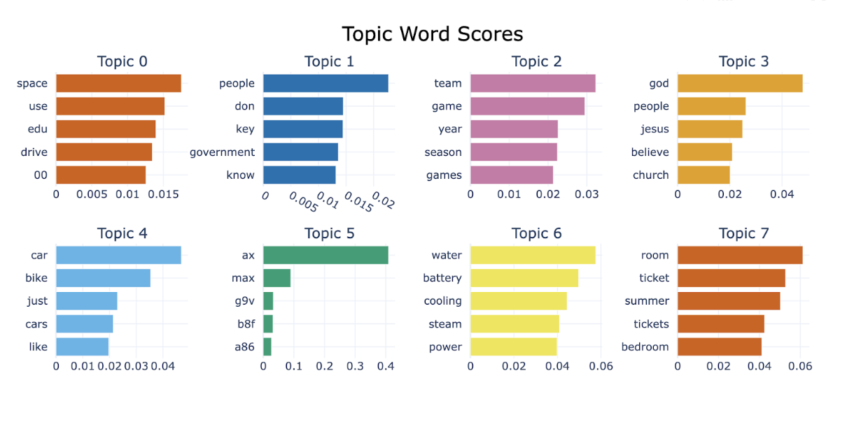
fig = topic_model.visualize_documents(docs)
fig.show()

LDA models word counts probabilistically and assumes documents are mixtures of topics. BERT-based topic modeling does not assume any generative process. Instead, it relies on semantic embeddings and clustering. LDA works well for short vocabularies and interpretable math. BERT-based topic modeling excels at capturing context, synonyms, and semantic similarity.

What is the difference between topic modelling and text classification? Topic modelling is unsupervised and discovers topics automatically without labeled data, while text classification is supervised and assigns predefined labels to documents based on training examples.

Can a document belong to more than one topic? Yes, most topic modelling methods assume that documents contain multiple topics, each with a certain probability or proportion.

How many topics should I choose? There is no fixed rule. The number of topics depends on the dataset size, domain, and use case. Experimentation and coherence evaluation are commonly used to find a suitable number.

Is topic modelling the same as clustering? Topic modelling and clustering are related but not identical. Clustering assigns each document to a single group, while topic modelling represents documents as mixtures of multiple topics.

Does topic modelling understand meaning? Topic modelling does not truly understand language in a human sense. It identifies statistical patterns in word usage, which often align well with human-interpretable themes.

Topic modelling is one of the essential algorithms that helps make sense of the growing volume of unstructured text data. Understanding hidden patterns through word co-occurrence allows us to move beyond surface-level keyword analysis and gain a more holistic understanding of large document collections. Approaches such as Latent Dirichlet Allocation, Non-negative Matrix Factorization, and Probabilistic Latent Semantic Analysis all tackle this challenge from different mathematical and probabilistic perspectives, offering flexibility depending on the nature of the data and the problem at hand.

While no single method works for all, choosing the right model and tuning it thoughtfully can reveal rich, interpretable insights that would be difficult to obtain manually. When used with domain knowledge and careful evaluation, topic modelling not only streamlines text analysis workflows but also serves as a powerful foundation for downstream tasks such as document clustering, information retrieval, and exploratory data analysis.